Mastering Reinforcement Learning

In 2020, I came across a YouTube video by Two Minute Papers on how a computer was able to learn to play a game of hide and seek on its own and even exploit a design flaw in the game engine to guarantee it always won. This discovery blew my mind but I didn’t think much of it. A few months later I was back in school for my penultimate year and decided to take on C++ as it was a requisite for getting a job as a Quant.

During this time and amid a very depressing semester break, I learnt about AlphaGo, the computer that learnt to play and become an expert in Go through self-play and even beat a World Champion. So, this time I did a little digging and found myself knee-deep in the rabbit hole of Machine Learning.

But beyond the beauty of Supervised and Unsupervised Learning, Natural Language Processing, Convolutional Neural Networks, and even the algorithms that learn to play games through self-play, my interest in Machine Learning was only piqued after I attended a Quant Finance/Financial Engineering seminar for undergrads and new grads and in one of the sessions, I learnt of how Reinforcement Learning is used in making decisions in Financial Markets.

At this point, I wanted in, mainly because I thought I’d make a lot of money. So I audited as many courses as possible, from Data Science to Time Series and Machine Learning algorithms, and I learnt them all. But to my disappointment, most of them never really talked much about Reinforcement Learning.

I later found a course dedicated to this topic but found it too hard to understand and gave up after the first week and I thought that was that. But then ChatGPT came out and everyone was talking big about LLMs. Then I found a tweet on the training process of this very special chatbot.

If you are familiar with LLMs, you know how the story goes. LLMs like GPT-2 and GPT-3, although very good at zero-shot tasks, were prone to hallucinations, producing abusive content and a lot of other issues carefully grouped as the misalignment problem. Reinforcement Learning with Human Feedback (RLHF) was the solution. Developed by the researchers at OpenAI, this 4-letter abbreviation solved the alignment problem (not completely) and changed the game.

I decided to write on RLHF and I did. With this renewed interest in Reinforcement Learning (RL), I decided to implement the paper “Playing Atari with Deep Reinforcement Learning” from scratch. While attempting to implement the code, I kept on running into “allocated memory” issues and finally gave up.

My goal with writing this article is to try to explain all that I learnt from this trying to implement the paper, taking a course on RL, reading a really old textbook from the 90s and every other source I learnt from. Due to the curse of knowledge, I can’t promise that this article is what you need to finally understand this topic as writing it is also my attempt at fully understanding it.

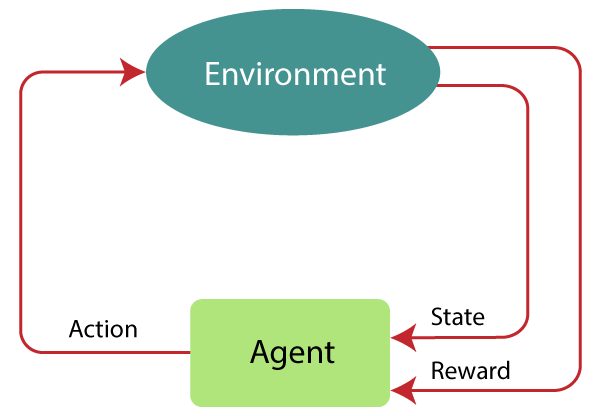
If you know anything about RL, then there’s a great chance you have seen a variant of the image. This image represents the “Typical RL scenario” where an Agent interacts with an environment by taking an action, gets a reward and a state which it uses to decide its next action. In this article, I don’t want to go the normal route by defining terms, and then moving on gradually. Instead, I want to answer the first question I had while taking the RL course, which is “How can I possibly train a computer to learn from experience and how complex is it”

Let’s dive in, shall we…

Breakout V.

Playing Atari with Deep Reinforcement Learning was my first stop on this journey. My goal was to implement the techniques outlined in the paper from scratch and teach my computer how to master Breakout, an Atari game. Among the five games presented in the paper, I chose Breakout due to my affinity for the game. My aspiration was to guide my computer to achieve the level of play depicted below:

The authors of the paper employed a variant of Q-learning for training.

But what exactly is Q-learning? According to Wikipedia:

Q-learning is a model-free reinforcement learning algorithm to learn the value of an action in a particular state. It does not require a model of the environment (hence "model-free"), and it can handle problems with stochastic transitions and rewards without requiring adaptations.

In essence, Q-learning is a reinforcement learning algorithm that aims to learn the value of taking a specific action in a particular state. The definition also points out that Q-learning is model-free, which means the algorithm works without having an in-depth knowledge of the environment beyond what it gets from state transitions after action selection.

Conversely, the counterpart to model-free algorithms is model-based algorithms. Most reinforcement learning algorithms fall under one of these two groups, although there are algorithms that use both approaches. Model-based algorithms unlike model-free algorithms require more knowledge of the environment like the reward function and state transition probabilities.

In the Q-learning algorithm, the agent's learning process hinges on observing state transitions and the corresponding rewards. This stands in contrast to model-based algorithms, which construct a detailed model of the environment's behaviour. This empowers model-based algorithms to simulate potential future scenarios, thereby facilitating informed decision-making based on accumulated knowledge.

In the case of using Q-learning for Breakout, the agent only observes the raw pixels from the game screen and takes action based on what is observed.

Similar to other branches of machine learning, the algorithm forms one piece of the larger puzzle. For instance, consider XGBoost, a traditional machine learning algorithm used for solving classification and regression problems related to tabular data analysis, Q-learning is a reinforcement learning algorithm used predominantly for solving problems modelled as Markov Decision Processes.

Returning to Wikipedia's definition of a Markov Decision Process (MDP):

a finite Markov decision process (MDP) is a discrete-time stochastic control process. It provides a mathematical framework for modeling decision making in situations where outcomes are partly random and partly under the control of a decision maker.

In the context of Atari games like Breakout, a Markov Decision Process captures the essence of the game. Each frame of the game serves as a discrete state, while the available actions represent the various moves the agent can make. The rewards reflect the points achieved in the game and the transitions model how the game environment evolves with each action taken.

Returning to the Q-learning algorithm…

The Q-learning algorithm is an optimization algorithm that aims to find the optimal action for any given state based on immediate rewards and the potential for higher rewards from future transitions. The algorithm aims to maximize the expected cumulative reward by approximating the value of all playable actions in each state and picking the action that has a maximum value.

Mathematically, this is ...

where, $Q^*(s, a)$ is a function of the state and action and is called the optimal action-value function,

$\mathbb{E}$ is used to denote expected value in math and statistics.

$R_t$ is the reward at timestep $t$.

$s_t$ is the current state,

$a_t$ is the action taken at timestep $t$, and

$\pi$ is the optimal policy.

The equation above is the optimal action-value function that estimates the expected cumulative reward for an action in a state given that the agent follows the optimal policy thereafter. The action-value function is denoted as, which is where the algorithm gets its name. It is called the Q-learning algorithm because it aims to learn and approximate the Q function.

In practice, the Bellman Equation is used to update the Q-function (action-value function) based on immediate rewards and discounted future rewards.

Bellman Equation

The Bellman Equation writes the "value" of a decision problem at a certain point in time in terms of the payoff from some initial choices and the "value" of the remaining decision problem that results from those initial choices.

In RL, the rewards for action are not always immediate and might even depend on future states. With the Bellman Equations, we can express the value of a state in terms of the reward obtained from the current action in that state and the anticipated rewards from future states. These future rewards are often discounted, meaning they are scaled by a discount factor (usually denoted as $\gamma$) that reflects the agent's preference for immediate versus future rewards. For instance, a discount factor of 0.99 indicates that the agent values future rewards at approximately 99% of immediate rewards.

The Bellman Equation is usually written for the value of a state (the state-value function) but can be adopted for the action-value function (which in this case, is what we need). The Bellman Equation for the action-value function is written as:

Here,

$s'$ is the next state that results from taking action $a$ in state $s$.

$r$ is the immediate reward obtained after taking action $a$ in state $s$ and transitioning to state $s'$.

$\text{max}_{a'}Q(s', a')$represents the maximum action-value achievable from state $s'$ onwards considering all possible actions $a'$ and their corresponding values. This can also be written as $Q^*(s', a')$, the optimal action-value function.

The Bellman Equation, therefore, provides a recursive equation for the action-value function.

Approximating the Q-value function

Similar to many optimization techniques, approximating the Q-value function is an iterative process. The Q-learning algorithm has an update rule for the Q-function given by

where $\alpha$ is the learning rate.

However, iterative algorithms necessitate assurance of convergence to a solution. This entails confirming whether continued Q-function adjustments at each timestep will eventually converge to the optimal action-value function.

In theory, the Q-value function would require a definition for every conceivable state-action pair. This is not feasible and the only option we are left with is to find a close estimate of the function. There are many methods for estimating the Q-value function. A traditional approach is to assume the function is linear and learn its parameters using gradient descent or the Normal Method (Least Squares).

However, this is suboptimal, as the Q-value function may not exhibit a linear relationship with states and actions. To overcome this limitation, Deep Neural Networks are employed for estimating the Q-value function. DNNs have demonstrated their capability in modelling nonlinear relationships using activations such as ReLU (Rectified Linear Unit) and sigmoid. This variant of Q-learning is sometimes called Deep Q-learning and is a part of Deep Reinforcement Learning algorithms.

The input to the Neural Network, known as a Deep Q-Network, comprises raw pixels from the gaming environment. These images are preprocessed and a Convolutional Neural Network learns the necessary features. The output layer consists of perceptrons, each corresponding to a possible action. A linear activation function is used to generate the Q-values for each action, given an input state.

Pseudo-code

Step...

1. Initialize Hyperparameters: Learning rate, Discount factor, Exploration probability (epsilon), Minimum exploration probability, Exploration decay, Target update frequency

2. Define Q-Network Architecture

3. Initialize Experience Replay: Use a deque (double-ended queue) to store experiences with a maximum capacity.

4. Define Action Selection Function: Create a function to choose actions based on the current state:
   • If a random number is less than the exploration probability, choose a random action.
   • Otherwise, select the action with the highest Q-value.

   This is the Exploration-Exploitation trade-off also called an epsilon-greedy policy

5. Main Training Loop:
   • Iterate through a fixed number of episodes (else training goes on forever)
   • Reset the environment to the initial state.
   • While the episode is not done:
     • Select an action based on the current state using the action selection function.
     • Take the selected action and observe the next state, reward, and whether the episode is done.
     • Store the experience (state, action, reward, next_state, done) in the experience replay buffer.
     • Sample a batch of experiences from the replay buffer.

6. Update Q-Values: For each experience in the batch:
   • Calculate the target Q-value based on the Bellman equation:
     • If the episode is not done, the target is the reward plus the discounted maximum Q-value of the next state.
     • If the episode is done, the target is just the reward.
   • Compute the current Q-value for the given state-action pair.
   • Update the Q-value using the learning rate and the Q-value update formula.

7. Decay Exploration Probability: Decay the exploration probability over time, gradually shifting from exploration to exploitation.

8. Move to Next State: Update the current state to the next state to continue the episode.

K-armed Bandits

In RL, a fundamental challenge arises when an agent must decide whether to rely on its existing knowledge to make decisions or to explore alternative actions in search of better strategies. This is known as the Exploration-Exploitation trade-off. Usually, an epsilon-greedy policy is used to get the right trade-off when training an agent.

To further explain this concept, I want to talk about the K-armed bandit's problem which I first encountered in a course on Coursera and I think has a pretty cool name. The K-armed bandit problem is also called the multi-armed bandit problem.

This problem is best described in a casino setting with slot machines. So, imagine you are faced with three slots, each offering rewards based on distinct probability distributions. Essentially, these machines yield rewards at different rates. For instance, the first machine might have a return rate of 0.2, implying a 20% chance of winning upon pulling its lever. The second and third machines might have probabilities of 30% and 45%, respectively. Importantly, the agent tasked with pulling these levers lacks any prior knowledge about these underlying probability distributions. The agent's objective is to maximize its cumulative reward over a series of pulls, which could range from 1000 to 10000, over time converging towards the probabilities through the law of large numbers.

While the optimal choice of which machine to pull might seem clear to us, the agent itself is oblivious to this information. As a result, it initially resorts to pulling each lever randomly, hoping to receive its first reward. If the initial reward emerges from, let's say, the first machine with the lowest probability, the agent faces a pivotal decision. t must decide whether to persistently exploit this newfound knowledge by repeatedly pulling that specific lever or to explore other levers in search of a potentially higher total reward.

The learning process typically commences with the agent choosing actions randomly in the early stages. As the agent accumulates more experience and insight into the environment, it gradually shifts its strategy towards exploiting its acquired knowledge, opting for actions that are currently deemed to yield higher expected rewards, rather than exploring random alternatives.

Crucially, the balance between exploration and exploitation hinges on a parameter epsilon ($\epsilon$). Epsilon assumes a value between 0 and 1, determining the agent's propensity to choose a random action. A higher epsilon, say 0.1, signifies a greater emphasis on exploration, as the agent frequently takes random actions to gather valuable information. Conversely, a lower epsilon, like 0.01, steers the agent towards exploitation, causing it to favour actions that have demonstrated promising outcomes based on its learned estimates.

Policy Gradients

Recently, I took up writing and published a few articles on Medium, one of which focused on Reinforcement Learning with Human Feedback. During my research, I encountered two papers that employed RLHF (Reinforcement Learning with Human Feedback) to address alignment issues in Language Model models (LLMs). Interestingly, both papers mentioned the utilization of the Proximal Policy Optimization (PPO) algorithm. However, they didn't delve deeply into the workings of the algorithm itself. My curiosity led me to explore the world of Policy Gradients and their significance in reinforcement learning.

Conventionally, many Reinforcement Learning algorithms learn the optimal policy by estimating a value function. This value function assigns values to actions based on the states they occur in, as demonstrated in Q-learning. Policy Gradients, in contrast, aim to learn the policy directly. Instead of focusing on a value function, they estimate a policy function.

The policy function denoted as $\pi(a|s, \theta)$, relies on the parameter vector $\theta$ to be learned. This function computes the probability of taking a specific action in a given state.

This is similar to value-functions like the Q-value function but in the equation, the weights are not usually added. The Q-value function can be written as $Q(s, a, w)$ where $w$ represents the weights or parameter vector.

To learn the optimal policy directly, the parameters of the policy function have to be updated in a way that converges to the optimum. The policy function is differentiated with respect to the parameters. The objective function/loss function is given by:

Here,

$\mathbb{E}_{r \sim \pi}$ represents the expectation taken over the rewards obtained by following a policy $\pi$

$\sum^{T}_{t=0}$ is a summation over time steps from $t=0$ to $t=T$, where $T$ is the time horizon of the episode.

$r(s_t, a_t)$ represents the reward obtained at time step $t$ when taking action $a_t$ in state $s_t$.

$\nabla_\theta \log \pi(a_t| s_t, \theta)$ is the gradient of the logarithm of the policy $\pi$ with respect to the policy parameters $\theta$, evaluated for action $a_t$ given state $s_t$. It signifies how the probability of selecting action $a_t$ changes with respect to changes in the policy parameters.

The use of the log of policy is a matter of convenience when differentiating the loss function, especially in chain rule which is common during back-propagation for Deep Neural Networks.

This strategy does have some limitations, with the obvious one being that optimization might get stuck in a local optimal. Others include high variance, where the gradient might have high fluctuations, leading to unstable learning and making the algorithm take longer to converge. This method also requires more sampling as unlike Q-learning, it does not use an experience replay but instead learns online and does gradient updates in a single batch after the episode ends.

To solve some of these issues, especially high variance, Trust Region Policy Optimization was introduced. TRPO places a constraint on the policy update to ensure that it remains within a certain "trust region," typically close to the old policy. This constraint is crucial for maintaining the stability of the learning process and preventing large policy updates that could lead to divergence. Here, the objective function is defined as:

Here,

$\mathbb{E}_{r \sim \pi_{old}}$ indicates an expectation taken over the rewards obtained by following the old policy $\pi_{old}$.

$\frac{\pi(a_t|s_t, \theta)}{\pi_{old}(a_t|s_t)}$ represents the likelihood ratio between the new policy $\pi$ and the old policy $\pi_{old}$ for taking action $a_t$ in state $s_t$. It measures how much the new policy has changed from the old policy for the specific action.

$A^{\pi_{old}}(s_t, a_t)$ is the advantage function under the old policy $\pi_{old}$, which quantifies the relative value of selecting action $a_t$ in state $s_t$ compared to the average action value.

The advantage function is usually defined as $A = Q - V$, with Q and V representing the Action-value and state-value functions respectively. The idea of using an advantage function was first introduced in the Actor-Critic algorithm which combines the strengths of policy gradient methods and value-based algorithms. In the Actor-Critic architecture, the actor updates the policy while the critic employs the advantage function to provide valuable feedback for policy improvement.

The Trust Region Policy Optimization (TRPO) method, while effective, is known for its complexity in implementation and the computational resources it demands. Constrained optimization, as employed by TRPO, can be challenging to implement. However, TRPO shines in delivering stable policy changes which is a crucial factor.

Enter the Proximal Policy Optimization (PPO) algorithm, which greatly improves on TRPO. PPO takes the foundation laid by TRPO and refines it, making it not only better but also more accessible in terms of implementation.

PPO achieves this through a cleverly designed loss function:

Here,

$\mathbb{E}_{t}$ indicates an expectation taken over time steps. In the context of PPO, this typically refers to taking expectations over trajectories or sequences of actions taken using the policy.

$r_t(\theta)$ represents the ratio of the probability of taking an action under the new policy $\pi_\theta$ to the probability of taking the same action under the old policy $\pi_{\text{old}}$. It's defined as $\frac{\pi_\theta(a_t|s_t)}{\pi_{\text{old}}(a_t|s_t)}$, where $a_t$ is the action taken at time step $t$ in state $s_t$.

$A_t$ is the advantage function at time step $t$, which quantifies how much better or worse an action is compared to the average action in the same state.

$\text{clip}(r_t(\theta), 1- \epsilon , 1+ \epsilon )$ is a clipping operation applied to the ratio $r_t(\theta)$. It restricts the ratio to be within a certain range to prevent large policy updates. The range is determined by the values $1 - \epsilon$ and $1 + \epsilon$.

The genius of PPO's design lies in the simplicity and effectiveness of the clipping operation at its core. This operation guarantees that policy updates stay within a controlled range, mitigating the risk of abrupt changes that can lead to instability.

In contrast, TRPO relies on unconstrained optimization and involves calculating the Kullback-Leibler (KL) Divergence—a measure of the difference between two probability distributions. Accurate computation of the KL-Divergence can be computationally intensive, leading to the need for approximations to make TRPO more practically implementable. Additionally, parameter updates in policy gradients are executed using Stochastic Gradient Ascent (SGA), where gradient changes are added to policy parameters—a unique approach compared to many other machine learning methods that employ Stochastic Gradient Descent (SGD), where gradient changes are subtracted to minimize objective functions. This distinction highlights the uniqueness of policy gradients in maximizing objectives.

In summary, Policy Gradient algorithms, with their focus on directly learning policies, offer a distinct approach compared to value-based algorithms. While they tend to excel in certain tasks, it's important to note that they don't always replace value-based algorithms. The choice between these approaches often depends on factors like the problem's nature, the availability of data, and computational resources. Policy Gradient algorithms are particularly advantageous when prior knowledge and human feedback play a significant role in the learning process, leveraging these valuable inputs to enhance performance.

Categorising RL Algorithms

Algorithms in Reinforcement Learning can be effectively categorized based on their key properties, leading to a structured understanding of their functionalities:

Learning Value and Policy Functions

Model-Free and Model-Based Approaches

On-Policy and Off-Policy Learning

Exploration Strategies

Temporal Difference and Monte Carlo Methods

These categories lead to cases where an algorithm can be model-free and require epsilon-greedy policy during training (like Q-learning).

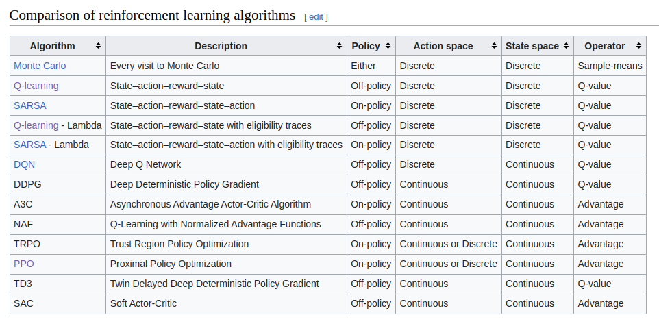
This table from Wikipedia shows the comparison of different reinforcement learning algorithms. These algorithms exhibit varying strengths and applicability, depending on the characteristics of the action and state spaces within an environment.

To clarify, the action space refers to the set of all possible actions an RL agent can take, while the state space encompasses all potential states the environment can assume. These spaces serve as the fundamental building blocks for RL algorithm selection.

For instance, the classic Q-learning algorithm excels in scenarios where the environment features a finite state space and a restricted set of actions. It leverages a Q-table to systematically evaluate state-action pairs, making it suitable for exhaustive exploration.

On the other hand, one of it’s variant, Deep Q-Network (DQN), emerges as a powerful choice when dealing with environments with infinite state spaces. DQN's strength lies in its utilization of deep learning techniques to approximate the Q-value function efficiently. However, it's essential to note that DQN still operates within a finite action space.

In essence, the compatibility between RL algorithms and the environment hinges on the dimensionality and nature of the action and state spaces. Understanding these spaces is pivotal in selecting the most appropriate algorithm for a given task. This adaptability empowers RL to address a diverse range of challenges, from problems with discrete, well-defined states to those featuring complex, high-dimensional state spaces in the real world.

Final Thoughts…

As we near the end of this journey and before I officially announce that I have said all I know about Reinforcement Learning, I’d like to say a few words about a new branch of Reinforcement Learning I discovered recently.

On some random twitter/X profile, I caught a glimpse into research in Inverse Reinforcement Learning. Inverse Reinforcement Learning (IRL)—or so I hope becomes the common name it's called—learns a reward function instead of a policy or action/state value function. This method has a lot of applications, especially in the real world (IRL) where the reward for behaviour is not easily known. This does sound like potentially interesting research and if I ever attempt getting a PhD in Computer Science or Mathematics, I would have to consider doing research.

For now, however, I have finished writing my article.

It’s pretty cool that I have already achieved my goal for writing this article and now have an in-depth understanding of reinforcement learning. I hope you do too and if you don’t, remember “Rome wasn’t built in a day” and maybe no one can fully understand reinforcement learning by reading one article.

References

Haarnoja, T. (2018, December 13). Soft Actor-Critic Algorithms and Applications. arXiv.org.

Mnih, V., Kavukcuoglu, K., Silver, D., Graves, A., Antonoglou, I., Wierstra, D., & Riedmiller, M.

Policy Gradient - Notes on AI. (n.d.). https://notesonai.com/Policy+Gradient#Policy+Gradient Proximal policy optimization. (n.d.). https://openai.com/research/openai-baselines-ppo Schulman, J. (2015, February 19). Trust Region Policy Optimization. arXiv.org.

Schulman, J. (2017, July 20). Proximal Policy Optimization Algorithms. arXiv.org.

Sutton, R. S., & Barto, A. G. (1998). Reinforcement learning: An Introduction. MIT Press.

Trust Region Policy Optimization — Spinning Up documentation. (n.d.).

Wikipedia contributors. (2023). Reinforcement learning. Wikipedia.

Use of Generative AI

I'd like to highlight my reliance on ChatGPT and Bard throughout this endeavour. I extensively utilized ChatGPT for editing my drafts and for gaining insights into the algorithms I discussed. Additionally, I engaged in valuable and insightful conversations with Bard especially on Bellman Equations. It's also worth mentioning that ChatGPT tends to apologise a lot lately.